Deep Learning
Step-by-step
- Why Deep Learning in AI ?
ImageNet challenge: It
is Olympics of computer vision!, Every year, researchers attempt to classify
images into one of 200 possible classes given a training dataset of
approximately 450,000 images.
The goal of the competition is to push the state of the art in computer vision
to rival the accuracy of human vision itself (approximately 95– 96%).
In 2012, Alex Krizhevsky at the University of Toronto did the unthinkable.
Pioneering a deep learning architecture known as a convolutional neural network
for the first time on a challenge of this size and complexity, he blew the
competition out of the water. The runner up in the competition scored a
commendable 26.1% error rate. But AlexNet, over the course of just a few months
of work, completely crushed 50 years of traditional computer vision research
with an error rate of approximately 16%
- Deep Learning core concepts
Neural General Function

Let’s reformulate the inputs as a vector x = [x1 x2 … xn]
and the weights of the neuron as w = [w1 w2 … wn].
Then we can re-express the output of the neuron as
y=f(x*w + b) , where b is the bias term.
In order to learn complex relationships, we need to use
neurons that employ some sort of nonlinearity. There are three major types of
neurons (Activation function) that are used in practice that introduce
nonlinearities in their computations (Sigmoid, Tanh, and ReLU Neurons).
Activation function (or non-linearity) : These activation functions take a single input and run
mathematical operations on it.
1) Sigmoid neurons: S-shaped nonlinearity, takes a real-valued
input and the output range from 0 to 1
σ(x)
= 1 / (1 + exp(−x))
2) Tanh neurons:
S-shaped nonlinearity, takes a real-valued input, and the output range
from −1 to 1
tanh(x)
= 2σ(2x) − 1
3) ReLU (Rectified
Linear Unit), It takes a real-valued input and thresholds it at zero (replaces
negative values with zero)
f(x) = max(0, x)

- Softmax Output Layers
it will show all output labels and how confident we are in
our predictions. the output depends on the outputs of all the other neurons.
So, if the input image ask if the content is dog or cat,
softmax layers at the end may answer with 0.9 cat, 0.1 dog
- Gradient Descent
In neural network, how exactly do we figure out the weights for
each node in neural network?
This is accomplished by training
t(i) is the true answer for the (i)th training example
y(i) is the value computed by the neural network,
we want to minimize the value of the error function E


E is zero when our model makes a perfectly correct
prediction on every training example. Moreover, the closer E is to 0, the
better our model is.
As a result, our goal will be to select our parameter vector θ (the values for
all the weights in our model) such that E is as close to 0 as possible.
use gradient descent algorithm to minimize the squared
error over all of the training examples.
But gradient descent algorithm may not
solve the problem if we have many local minimum

Should Local minima solved and find true global
minimum?
No, in most cases, no need to overcome Local minimum problem!
However, in case your network is stuck in a bad local minimum then you need to
tune your hyper parameters. You could try some of the following methods:
1) Increasing the learning rate: If the learning rate of your algorithm is too small
then it is more likely to be stuck in a local minima.
2) Increasing hidden layers/units: It may help approximate the
function better.
3) Trying different activation functions: Make sure that the
combination of activation functions is apt for your model and dataset.
4) Trying different optimization algorithms: Instead of the
conventional gradient descent, try using algorithms like Adam’s optimizer and
RMSProp, Adagrad, Adadelta, RMSprop, and SGD
- Difference between Back-propagation and Feed-forward
Neural Network
– Feed forward is algorithm to calculate output vector from
input vector.
– Back propagation is algorithm to adjust weight of neural network.
During training of neural network, all types of networks
using Feed Forward and Backpropagation Algorithms
In production, it is optional to use Back propagation
Feed Forward Neural Networks
use back-propagation during training time only
In these types of neural networks information flows in only one direction i.e.
from input layer to output layer.
When the weights are once decided, they are not usually changed.
The nodes here do their job without being aware whether results produced are
accurate or not(i.e. they don’t re-adjust according to result produced).
There is no communication back from the layers ahead.
Feed Forward Limitations:
– Can’t handle sequential data
– Considers only the current input
– Can’t memorize previous inputs
Recurrent Neural Networks (Back-Propagating)
use back-propagation during training time and production use. also Information
passes from input layer to output layer to produce result. Error in result is
then communicated back to previous layers now.
Nodes get to know how much they contributed in the answer being wrong. Weights
are re-adjusted. Neural network is improved. It learns.
There is bi-directional flow of information. This basically has both algorithms
implemented, feed-forward and back-propagation.
- Popular Neural Networks
- Multilayer Perceptrons (MLPs) OR Feed Forward Neural Network: Used in general
Regression and Classification problems
- Convolutional Neural Networks (CNNs) : Used for Image Recognition
- Recurrent Neural Networks (RNNs) : Used for Speech Recognition
- Deep Belief Network:
Used for Cancer Detection
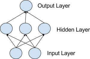
- Multilayer Perceptrons (MLPs)
class of feedforward artificial neural network (ANN)
it is a classical type of neural network. They are comprised
of one or more layers of neurons. Data is fed to the input layer, there may be
one or more hidden layers providing levels of abstraction, and predictions are
made on the output layer, also called the visible layer.
They are very flexible and can be used generally to learn a
mapping from inputs to outputs.
This flexibility allows them to be applied to other types of
data. For example, the pixels of an image can be reduced down to one long row
of data and fed into a MLP. The words of a document can also be reduced to one
long row of data and fed to a MLP. Even the lag observations for a time series
prediction problem can be reduced to a long row of data and fed to a MLP.
Use MLPs For:
- Tabular datasets
- Classification prediction problems
- Regression prediction problems
for
example, a dataset of gray scale images with the standardized size
of 32×32 pixels each, a traditional feedforward neural network would require
1024 input weights (plus one bias).
This is fair enough,
but the flattening of the image matrix of pixels to a long vector of pixel
values loses all of the spatial structure in the image. Unless all of the
images are perfectly resized, the neural network will have great difficulty
with the problem.
- RNN
RNN is a neural network with memory (It can memorize
previous inputs to help in predict the next)
So, RNN works on the principle of saving the output of a
layer and feeding this back to the input in order to predict the output of the
layer.
RNN can be used in NLP, Time Series Prediction, Machine
Translation, etc.
RNN types :
– One-to-One:
known as Vanilla NN, An observation as input mapped to one output
– One-to-Many: An observation as input mapped to a sequence with
multiple steps as an output. for example an image can convert to dog catch a
ball
– Many-to-One: A sequence of multiple steps as input mapped to class or
quantity prediction. for example in sentimental analysis many works feed to
classify it as positive or negative
– Many-to-Many: A sequence of multiple steps as input mapped to a
sequence with multiple steps as output. for example machine translation, many
words in input mapped to many words in output
But we may face gradient problem (Vanishing or Exploding)


while traning a RNN, Slope (Loss of
information through time) can be either too small or very large and this makes
training difficult.
Exploding Gradient Problem:
when the slope too heigh
Vanishing Gradient Problem: when the slope too small
Issue in Gradient Problem
– Long training time
– Poor performance
– Bad accuracy
Solution for Exploding Gradient Problem:
1) Identity Initialization
2) Truncated Backpropagation
3) Gradient Clipping
Solution for Vanishing Gradient Problem:
1) Weight Initialization
2) Choosing the right activation function
3) Long Short-Term Memory Network (LSTMs)
The Long Short-Term Memory (LSTM) network is perhaps the most successful RNN because it
overcomes the problems of training a recurrent network and in turn has been
used on a wide range of applications.
A Recurrent Neural Network looks something like this:

- CNN (Convolutional Neural Networks, also called
ConvNet)
CNN is a feed forward neural network that is generally used
for Image recognition and object classification.
Used for object recognition tasks such as handwritten digit
recognition.
CNN considers only the current input
CNN has 4 layers namely: Convolution layer, ReLU layer,
Pooling and Fully Connected Layer. Every layer has its own functionality and
performs feature extractions and finds out hidden patterns.
Below is an example of how CNN looks like:

- CNN vs RNN Summary
CNN is a feed forward neural network that is generally used
for Image recognition and object classification.
While RNN works on the principle of saving the output of a
layer and feeding this back to the input in order to predict the output of the
layer.
CNN considers only the current input
while RNN considers the current input and also the previously received inputs.
It can memorize previous inputs due to its internal memory.
RNN can handle sequential data while CNN cannot.
In RNN, the previous states is fed as input to the current
state of the network. RNN can be used in NLP, Time Series Prediction, Machine
Translation, etc.
CNN has 4 layers namely: Convolution layer, ReLU layer,
Pooling and Fully Connected Layer. Every layer has its own functionality and
performs feature extractions and finds out hidden patterns.
There are 4 types of RNN namely: One to One, One to Many,
Many to One and Many to Many.
(because RNNs has designed to work with sequence prediction problems)
Use CNNs For:
- Image data
- Classification prediction problems (document
classification / sentiment analysis )
- Regression prediction problems
- Text data
- Time series data
- Sequence input data
Use RNNs For:
- Text data
- Speech data
- Classification prediction problems
- Regression prediction problems
- Generative models
Don’t Use RNNs For:
- Tabular data
- Image data
- COCO Dataset (Common Objects In Context Dataset)
To train Deep Learning network to detect an object, we need
lots of pictures of the kinds objects that we want to detect.
to save time, there are a several public datasets of images already exist.
There’s a popular dataset called COCO (short for Common Objects In Context)
that has images annotated with object masks.
In this dataset, there are over 12,000 images
COCO model knows how to detect 80 different common objects,
Here is a full list of them.
class_names = ['BG', 'person',
'bicycle', 'car', 'motorcycle', 'airplane',
'bus', 'train', 'truck', 'boat',
'traffic light',
'fire hydrant', 'stop sign', 'parking
meter', 'bench', 'bird',
'cat', 'dog', 'horse', 'sheep', 'cow',
'elephant', 'bear',
'zebra', 'giraffe', 'backpack',
'umbrella', 'handbag', 'tie',
'suitcase', 'frisbee', 'skis',
'snowboard', 'sports ball',
'kite', 'baseball bat', 'baseball
glove', 'skateboard',
'surfboard', 'tennis racket', 'bottle',
'wine glass', 'cup',
'fork', 'knife', 'spoon', 'bowl',
'banana', 'apple',
'sandwich', 'orange', 'broccoli', 'carrot',
'hot dog', 'pizza',
'donut', 'cake', 'chair', 'couch',
'potted plant', 'bed',
'dining table', 'toilet', 'tv',
'laptop', 'mouse', 'remote',
'keyboard', 'cell phone', 'microwave',
'oven', 'toaster',
'sink', 'refrigerator', 'book', 'clock',
'vase', 'scissors',
'teddy bear', 'hair drier',
'toothbrush']
- YOLO3 for Image processing
CNN Limitation
CNN (2012) goes pixle by pixle to detect an object, also
have to scan the same image multiple times to detect all objects and this
consume alot of time
CNN has been improved over years, R-CNN (2013) , Fast R- CNN
(2015) , Faster R-CNN (2015), and Mask R-CNN (2017)
[ Mask R-CNN extending Faster R-CNN techniques and aim to locate exact pixels
of each object instead of just bounding boxes]
While R-CNN family tend to very accurate, the biggest
problem with the R-CNN family of networks is their speed
they were incredibly slow, obtaining only 5 FPS on a GPU.
To help increase the speed of deep learning-based object
detectors, YOLO (2015) use a one-stage detector strategy.
Yolo algorithm treat object detection as a regression problem, taking a given
input image and simultaneously learning bounding box coordinates and
corresponding class label probabilities.
YOLO2 capable of detecting over 9,000 object detectors. can
obtaining 45 FPS on a GPU.
YOLO2 able to achieve such a large number of object
detections by performing joint training for both object detection and
classification. Using joint training the authors trained YOLO9000
simultaneously on both the ImageNet classification dataset and COCO detection
dataset. The result is a YOLO model, called YOLO9000, that can predict
detections for object classes that don’t have labeled detection data.
while YOLO2 can detect 9,000 separate classes, the accuracy
is not quite what we would desire.
Yolo3 (2018):
a newer deep learning approach, that combines the
accuracy of CNNs with clever design and efficiency tricks that greatly speed up
the detection process. This will run relatively fast (on a GPU) as long as we
have a lot of training data to train the model.
YOLO object detection algorithm
YOLO take an image and split it into an SxS grid, within each of the grid we
take m bounding boxes. For each of the bounding box, the network outputs a
class probability and offset values for the bounding box. The bounding boxes
having the class probability above a threshold value is selected and used to
locate the object within the image.

Limitation and drawback of the YOLO object detector :
1) It does not always handle small objects well
2) It especially does not handle objects grouped close together
The reason for this limitation is due to the YOLO algorithm itself:
The YOLO object detector divides an input image into an SxS
grid where each cell in the grid predicts only a single object.
If there exist multiple, small objects in a single cell then YOLO will be
unable to detect them, ultimately leading to missed object detections.
Therefore, if you know your dataset consists of many small objects grouped
close together then you should not use the YOLO object detector.
In terms of small objects, Faster R-CNN tends to work the
best; however, it’s also the slowest.
Example of YOLO limitation: YOLO can detect only one of
the two wine glasses

Guidelines when picking an object detector for a given
problem:
– need to detect small objects and speed is not a
concern, use Faster R-CNN.
– speed is absolutely paramount, use YOLO.
– need balance between the YOLO/Faster R-CNN, use SSDs or RetinaNet
YOLO implementations
Currently there are 3 main implementations of YOLO, each one
of them with advantages and disadvantages
1) Darknet (https://pjreddie.com/darknet/).
This is the “official” implementation, created by the same people behind the
algorithm. It is written in C with CUDA, hence it supports GPU computation. It
is actually a complete neural network framework, so it really can be used for
other objectives besides YOLO detection. The disadvantage is that, since it is
written from the ground up (not based on a stablished neural network framework)
it may be more difficult to find answers for errors.
2) AlexeyAB/darknet (https://github.com/AlexeyAB/darknet).
it is actually a fork of Darknet to support Windows and Linux. it is an
excellent source to find tips and recommendations about YOLO in general, how to
prepare you training set, how to train the network, how to improve object
detection, etc.
3) Darkflow (https://github.com/thtrieu/darkflow/).
This is port of Darknet to work over TensorFlow. This is the system I have used
the most, mainly because I started this project without having a GPU to train
the network and apparently using CPU-only Darkflow is several times faster than
the original Darkent. AFAIK the main disadvantage is that it has not been
updated to YOLOv3.
All these implementations come “ready to use”, which means
you only need to download and install them to start detecting images or videos
right away using already trained weights available to download. Naturally this
detection will be limited to classes contained in the datasets used to obtain
this weights.
- Sample YOLO script in Python to detect Objects
Before run the next code you need to install Python x64
from https://www.python.org/downloads/
then open command line as an Administrator and run the next two commands
pip install numpy
pip install opencv-python
Python code to detect objects using OpenCV library
# USAGE
# python yolo.py --image
images/baggage_claim.jpg
# import the necessary packages
import numpy as np
import argparse
import time
import cv2
import os
# construct the argument parse and parse
the arguments
ap = argparse.ArgumentParser()
ap.add_argument("-i",
"--image", required=True, help="path to input image")
ap.add_argument("-c",
"--confidence", type=float, default=0.5, help="minimum
probability to filter weak detections")
ap.add_argument("-t",
"--threshold", type=float, default=0.3, help="objects Overlap less than,
normally between 0.3 and 0.5")
args = vars(ap.parse_args())
YoloConfigDirectory="yolo-coco"
# derive the paths to the YOLO weights
and model configuration
weightsPath =
os.path.sep.join([YoloConfigDirectory, "yolov3.weights"])
configPath =
os.path.sep.join([YoloConfigDirectory, "yolov3.cfg"])
# load the COCO class labels our YOLO
model was trained on
labelsPath =
os.path.sep.join([YoloConfigDirectory, "coco.names"])
LABELS = open(labelsPath).read().strip().split("\n")
# initialize a list of colors to
represent each possible class label
np.random.seed(42)
COLORS = np.random.randint(0, 255,
size=(len(LABELS), 3), dtype="uint8")
# load our YOLO object detector trained
on COCO dataset (80 classes)
print("[INFO] loading YOLO from
disk...")
net =
cv2.dnn.readNetFromDarknet(configPath, weightsPath)
# load our input image and grab its
spatial dimensions
image =
cv2.imread(args["image"])
(H, W) = image.shape[:2]
# determine only the *output* layer
names that we need from YOLO
ln = net.getLayerNames()
ln = [ln[i[0] - 1] for i in
net.getUnconnectedOutLayers()]
# construct a blob from the input image
and then perform a forward
# pass of the YOLO object detector, giving
us our bounding boxes and
# associated probabilities
blob = cv2.dnn.blobFromImage(image, 1 /
255.0, (416, 416), swapRB=True, crop=False)
net.setInput(blob)
start = time.time()
layerOutputs = net.forward(ln)
end = time.time()
# show timing information on YOLO
print("[INFO] YOLO took {:.6f}
seconds".format(end - start))
# initialize our lists of detected
bounding boxes, confidences, and
# class IDs, respectively
boxes = []
confidences = []
classIDs = []
# loop over each of the layer outputs
for output in layerOutputs:
# loop over each of the
detections
for detection in output:
# extract the
class ID and confidence (i.e., probability) of the current object detection
scores =
detection[5:]
classID =
np.argmax(scores)
confidence =
scores[classID]
# filter out
weak predictions by ensuring the detected
# probability is
greater than the minimum probability
if confidence
> args["confidence"]:
#
scale the bounding box coordinates back relative to the
#
size of the image, keeping in mind that YOLO actually
#
returns the center (x, y)-coordinates of the bounding
#
box followed by the boxes' width and height
box
= detection[0:4] * np.array([W, H, W, H])
(centerX,
centerY, width, height) = box.astype("int")
#
use the center (x, y)-coordinates to derive the top and
#
and left corner of the bounding box
x =
int(centerX - (width / 2))
y =
int(centerY - (height / 2))
#
update our list of bounding box coordinates, confidences,
#
and class IDs
boxes.append([x,
y, int(width), int(height)])
confidences.append(float(confidence))
classIDs.append(classID)
#Apply “non-max suppression” that
eliminate possible duplicate objects and leave the most exact of them
idxs = cv2.dnn.NMSBoxes(boxes,
confidences, args["confidence"], args["threshold"])
# ensure at least one detection exists
if len(idxs) > 0:
# loop over the indexes we
are keeping
for i in idxs.flatten():
# extract the
bounding box coordinates
(x, y) =
(boxes[i][0], boxes[i][1])
(w, h) =
(boxes[i][2], boxes[i][3])
# draw a
bounding box rectangle and label on the image
color = [int(c)
for c in COLORS[classIDs[i]]]
cv2.rectangle(image,
(x, y), (x + w, y + h), color, 2)
text = "{}:
{:.4f}".format(LABELS[classIDs[i]], confidences[i])
cv2.putText(image,
text, (x, y - 5), cv2.FONT_HERSHEY_SIMPLEX, 0.5, color, 2)
# show the output image
cv2.imshow("Image", image)
cv2.waitKey(0)
This code assume that we have a folder in the same python
script path with name “yolo-coco” contains 3 files, these files are a model
files (pre-trained object detector on the COCO dataset)

Python Script takes 3 parameters:
–image : The path to the input image. We’ll detect objects in this
image using YOLO.
–confidence : Minimum probability to filter weak detections.
default value is 0.5
–threshold : This is our non-maxima suppression threshold with a
default value of 0.3
tune threshold to avoid detect the same
object many time

Here is the script result after run and feed with one image

Read Sourcecode from
https://github.ibm.com/MRAFIE/DeepLearning
Download the complete souce code from
https://drive.google.com/file/d/1MwOKO7DIH_gckT5QO35qTH_O6DnFRVC4/view?usp=sharing
- What are the Best Free Image Datasets for Computer
Vision?
Google has released its open-source image dataset “Open
Image V5” in 2019 to become the most big and free dataset availabe now
contains ~9 million images that have been annotated with labels spanning over
6,000 categories, for more information about dataset and how to get it please
visit https://storage.googleapis.com/openimages/web/index.html
Other Image Datasets for Computer Vision Training
1) Visual Genome: (convert image to words)
Visual Genome is a dataset and knowledge base created in an effort to connect
structured image concepts to language. The database features detailed visual
knowledge base with captioning of 108,077 images.

2) VisualQA: VQA
is a dataset containing open-ended questions about 265,016 images. These
questions require an understanding of vision and language. So, we can ask “How
many children are in the bed?” or “Where is the child sitting?”

3) CelebFaces:
Face dataset with more than 200,000 celebrity images, each with 40 attribute
annotations (Like Wavy Hair, Smile, Mustache…)

4) CompCars: Contains 163 car makes with 1,716 car models, with each car
model labeled with five attributes, including maximum speed, displacement,
number of doors, number of seats, and type of car.

5) Indoor
Scene Recognition: A very specific dataset. Contains
67 Indoor categories (Like detect Store, Work Place, Home, Public Space), and a
total of 15620 images.

6) Labelled Faces in the
Wild: 13,000
labeled images of human faces, for use in developing applications that involve
facial recognition to get the personal name of person after capture his image.

7) Stanford
Dogs Dataset: Contains
20,580 images and 120 different dog breed categories, with about 150 images per
class.

8) Places: Scene-centric database with
205 scene categories and 2.5 million images with a category label, can detect
indoor, outdoor,open area, natural light, clouds, sunny,…

9) Flowers: Dataset of images of flowers
commonly found in the UK consisting of 102 different categories. Each flower
class consists of between 40 and 258 images with different pose and light variations.

10) Plant Image Analysis: A collection of datasets spanning over 1 million images of
plants. Can choose from 11 species of plants.

11) Home Objects: A dataset that contains random objects from home, mostly
from kitchen, bathroom and living room split into training and test datasets.

- What is the Deep Learning Tools?
PyTorch is a machine learning and deep learning tool
developed by Facebook’s artificial intelligence division to process large-scale
image analysis, including object detection, segmentation and classification.
the other available tools are TensorFlow (developed by google), Theano (by
University of Montreal), Caffe, Neon, and Keras.
Google announced TensorFlow 2.0 in June 2019, they declared
that Keras is now the official high-level API of TensorFlow for quick and easy
model design and training.
Most of 2019 researchs use PyTorch while most of production
products use TensorFlow.
What about OpenCV?
it is a famous computer vision and machine learning library contains more than
2500 optimized algorithms.
but OpenCV does not provide any way to train a DNN. However,
you can train a DNN model using frameworks like Tensorflow, PyTorch etc, and
import it into OpenCV for your application.
What about OpenVINO?
it is specifically designed to speed up networks used in visual tasks like
image classification and object detection.
What is the role of hardware companies in the rise of AI?
When we think of AI, we usually think about companies like IBM, Google,
Facebook.. etc.
Well, they are indeed leading the way in algorithms but AI is computationally
expensive during training as well as inference.
Therefore, it is equally important to understand the role of hardware companies
in the rise of AI.
NVIDIA provides
the best GPUs as well as the best software support using CUDA and cuDNN for
Deep Learning.
NVIDIA pretty much owns the market for Deep Learning when it comes to training
a neural network.
However, GPUs are expensive and not always necessary for
inference (inference means use trained model on production).
In fact, most of the inference in the world is done on CPUs!
In the inference space, Intel is a big
player, it manufactures Vision Processing Units (VPUs), integrated GPUs, and
FPGAs — all of which can be used for inference.
and to avoid confusing developers about how to write code to
optimize the use of HW, Intel provides us OpenVINO framework
OpenVINO enables CNN-based deep learning inference on the
edge, supports heterogeneous execution across computer vision accelerators,
speeds time to market via a library of functions and pre-optimized kernels and
includes optimized calls for OpenCV and OpenVX.
How to use OpenVINO?
1) OpenCV or OpenVINO does not provide you tools to train a
neural network. So, train your model using Tensorflow or pytorch.
2) The model obtained in the previous step is usually not optimized for
performance.
OpenVINO requires us to create an optimized model which they
call Intermediate Representation (IR) using a Model Optimizer tool they
provide.
The result of the optimization process is an IR model. The model is split into
two files:
– model.xml : This XML file contains the network architecture.
– model.bin : This binary file contains the weights and biases.
3) OpenVINO Inference Engine plugin : OpenVINO optimizes
running this model on specific hardware through the Inference Engine plugin
- TensorFlow vs PyTorch
• In TensorFlow, we have to define the tensors, initialize
the session, and keep placeholders for the tensor objects; however, we do not
have to do these operations in PyTorch.
• In TensorFlow, let’s consider sentiment analysis as an
example. Input sentences are tagged with positive or negative tags. If the
input sentence’s length is not equal, then we set the maximum sentence length
and add zero to make the length of other sentences equal, so that the recurrent
neural network can function; however, this is a built-in functionality in PyTorch,
so we do not have to define the length of the sentences.
• In PyTorch, the debugging is much easier and simpler, but
it is a difficult task in TensorFlow.
In 2019, PyTorch has the research market, and is trying to
extend this success to industry. TensorFlow is trying to stem its losses in the
research community without sacrificing too much of its production capabilities.
Why industry use TensorFlow instead of PyTorch?
No Python.
Some companies will run servers for which the overhead of the Python runtime is
too much to take.
Mobile. You can’t embed a Python interpreter in your mobile binary.
Serving. A catch-all for features like no-downtime updates of
models, switching between models seamlessly, batching at prediction time, and
etc.
TensorFlow was built specifically around industry
requirements, and has solutions for all these issues: the graph format and
execution engine natively has no need for Python, and TensorFlow Lite and
TensorFlow Serving address mobile and serving considerations respectively.
How TensorFlow and PyTorch address there weaknesses?
PyTorch introduced
the JIT compiler: support deploy PyTorch models in C++ without a Python
dependency, also announced support for both quantization and mobile.
TensorFlow moving
to eager mode in v2.0 : At the API level, TensorFlow eager mode is essentially
identical to PyTorch’s eager mode.
This gives TensorFlow most of the advantages of PyTorch’s eager mode (ease of
use, debuggability, and etc.)
However, this also gives TensorFlow the same disadvantages. TensorFlow eager
models can’t be exported to a non-Python environment, they can’t be optimized,
they can’t run on mobile, etc.
This puts TensorFlow in the same position as PyTorch.
But TensorFlow Eager suffers heavily from performance/memory issues till now.
- How to install PyTorch?
pip3 install torch torchvision
or
pip3 install torch==1.3.0+cpu torchvision==0.4.1+cpu -f
https://download.pytorch.org/whl/torch_stable.html
Notes
to get the latest installation command visit https://pytorch.org/
form the blow image, user will choose his OS and Python
version to get the installation command

by RafieTarabay